- 41patients segmented, 16 LV segments each
- 85%of LGE elevations also detected by T1ρ
- 0.480strongest correlation (T2 vs. T1ρ)
- 0.047weakest (ECV vs. T1ρ, LGE-positive only)
Myocardial fibrosis is a cardiac disease where scar tissue forms in the heart muscle (myocardium) after an injury, such as an infarction. The scar tissue can stiffen the myocardium and lead to heart failure.
The disease can be diagnosed from images produced by Magnetic Resonance Imaging (MRI). An MRI of the heart is called Cardiovascular Magnetic Resonance (CMR). Different measurements yield different maps, and these maps vary in how well they diagnose fibrosis. Late gadolinium-enhanced imaging (LGE) is a valid clinical reference. It requires injection of a gadolinium-based contrast agent (GBCA) to increase tissue contrast.
Why an alternative is needed
GBCA may cause nephrogenic systemic fibrosis in patients with renal disease. They are not recommended for pregnant patients. They can also cause minor side effects, such as nausea and headaches, and in rare cases allergic reactions. These groups cannot safely receive a GBCA injection, so a contrast-free method is needed.
T1ρ is a promising contrast-free technique, but further evidence is needed to support its effectiveness. The aim of this project was to compare T1ρ against the contrast-based maps used in the clinic, and against the standard contrast-free map, to evaluate whether it can act as an alternative.
The maps
MRI uses a strong static magnetic field, referred to as B0, together with radiofrequency (RF) pulses. The maps are time measurements, based on the alignment of the precession of spin of hydrogen nuclei. Each map is sensitive to something different.
T1 is the longitudinal relaxation time, i.e., the time it takes for the precession of hydrogen nuclei to realign with B0 after being excited by an RF pulse.
T2 is the relaxation time in the transverse component of the net magnetization. Hydrogen nuclei in different chemical environments do not precess at the same frequency, so the spins dephase and the transverse component decays. T2 yields higher values when water volume increases, which can indicate inflammation.
T1ρ also measures a longitudinal relaxation time, but against a different magnetic field. An RF pulse tips the net magnetization 90 degrees into the transverse plane. A spin-lock RF pulse of amplitude B1 then holds the spins there. T1ρ is the time measured for relaxation within the transverse plane, as the amplitude of B1 decreases and the spins dephase. T1ρ is particularly sensitive to water–macromolecule interactions, so it shows increased values when extracellular matrix is present. This is the reason it is expected to detect fibrosis.
The two contrast-based maps in this study were LGE, where the contrast agent accumulates in scar tissue, and the extracellular volume fraction (ECV) of the myocardium.
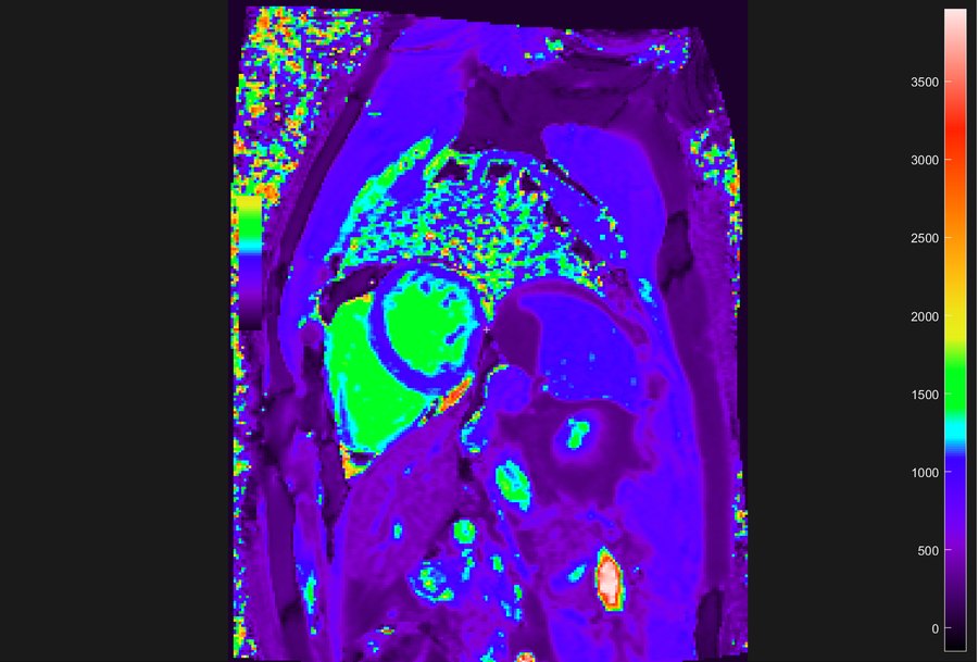
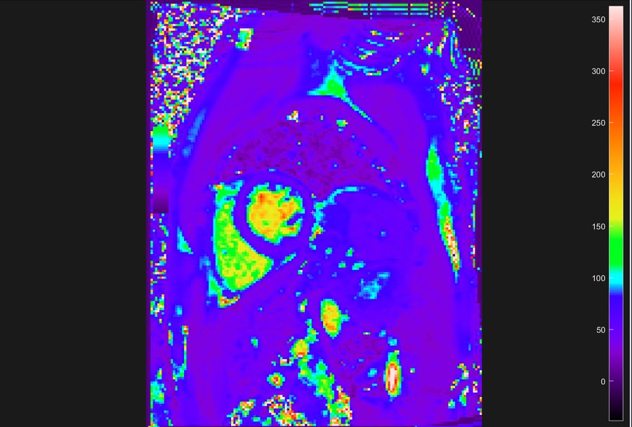
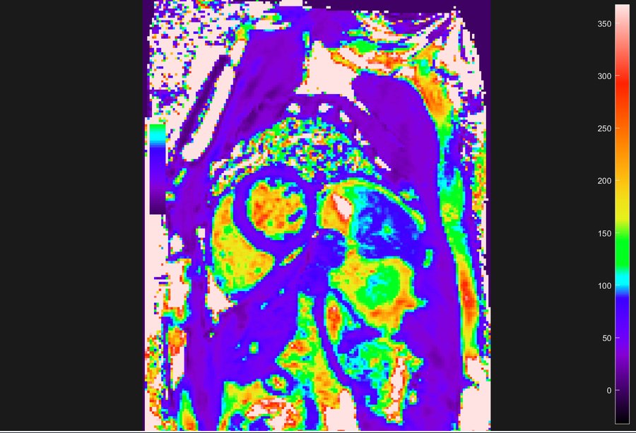
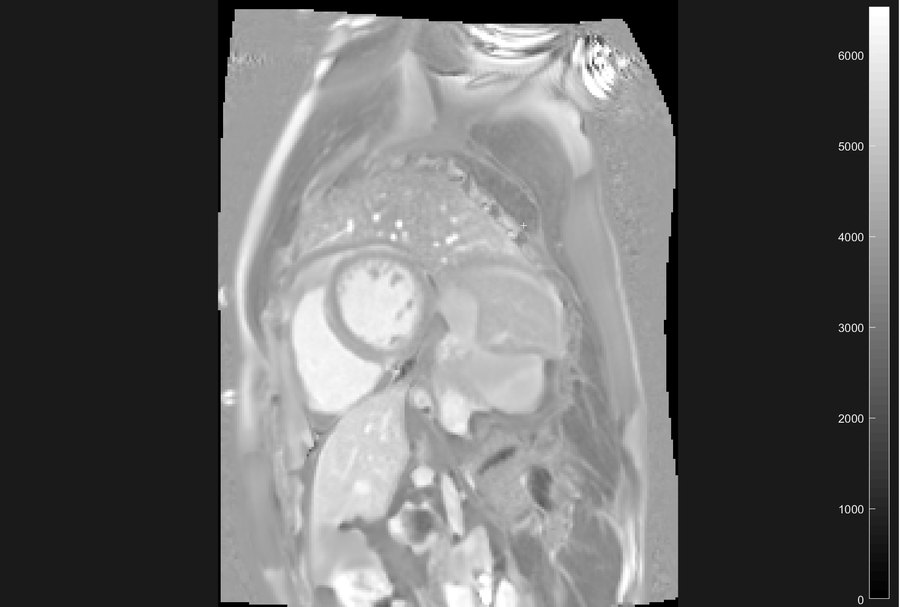
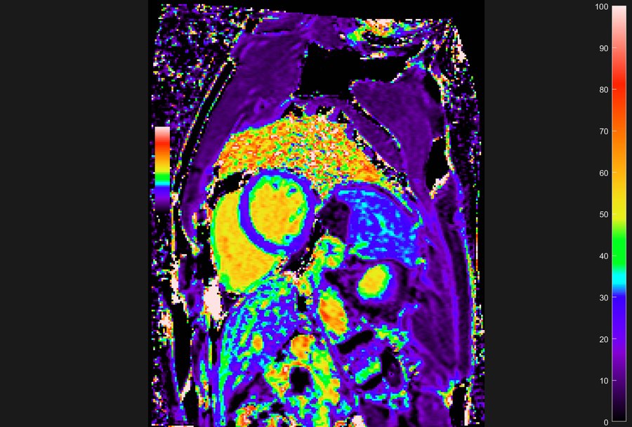
Reference values for healthy tissue
Fibrotic tissue appears as increased relaxation-time values. At a field strength of 1.5 T, there are fixed values that represent healthy myocardial tissue.
- T1ρ
- 54.2 ± 2.56 ms (presented at ISMRM, May 2026)
- T2
- 52.18 ± 3.4 ms
- ECV
- 20.4% to 30.4%
A value above the healthy range is an elevation. An elevation is not specific to myocardial fibrosis, since many conditions raise these values.
Left ventricular segmentation
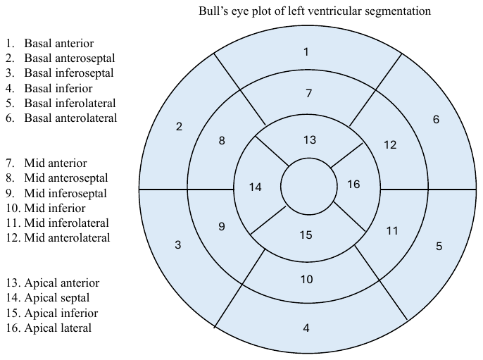
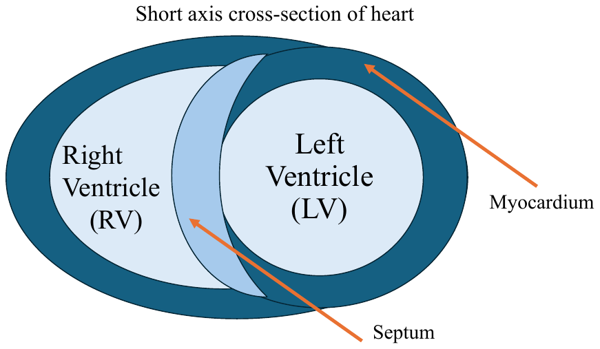
Comparing maps quantitatively requires comparing the same piece of muscle in each of them. The American Heart Association (AHA) describes a standard nomenclature for left ventricular (LV) segmentation. The LV is sliced parallel to the short axis into three layers: basal, mid-cavity and apical. Each layer is then divided into smaller segments. The AHA model uses 17 segments. This study excluded the apex (segment 17), which yields 16 segments.
Method
Pre-reconstructed in vivo CMRs of 41 patients were used. The MRIs were performed on a 1.5 T Siemens scanner. The data set included the maps ECV, T2 and T1ρ.
- Field strength
- 1.5 T Siemens
- Field of view
- 360–500 mm
- In-plane resolution
- 1.40–1.95 mm
- T1ρ spin lock
- 500 Hz, in 10 ms steps to a total of 40 ms
- Analysis software
- Segment Research by Medviso
Data acquisition through segmentation
Semi-automated 16-part segmentation was performed with the built-in bullseye plot tool in Segment Research. A perpendicular line through the center of the septum was marked as a reference for the software. The epicardial border was then eroded inward by 10% and the endocardial border outward by 10%, to exclude blood pools.
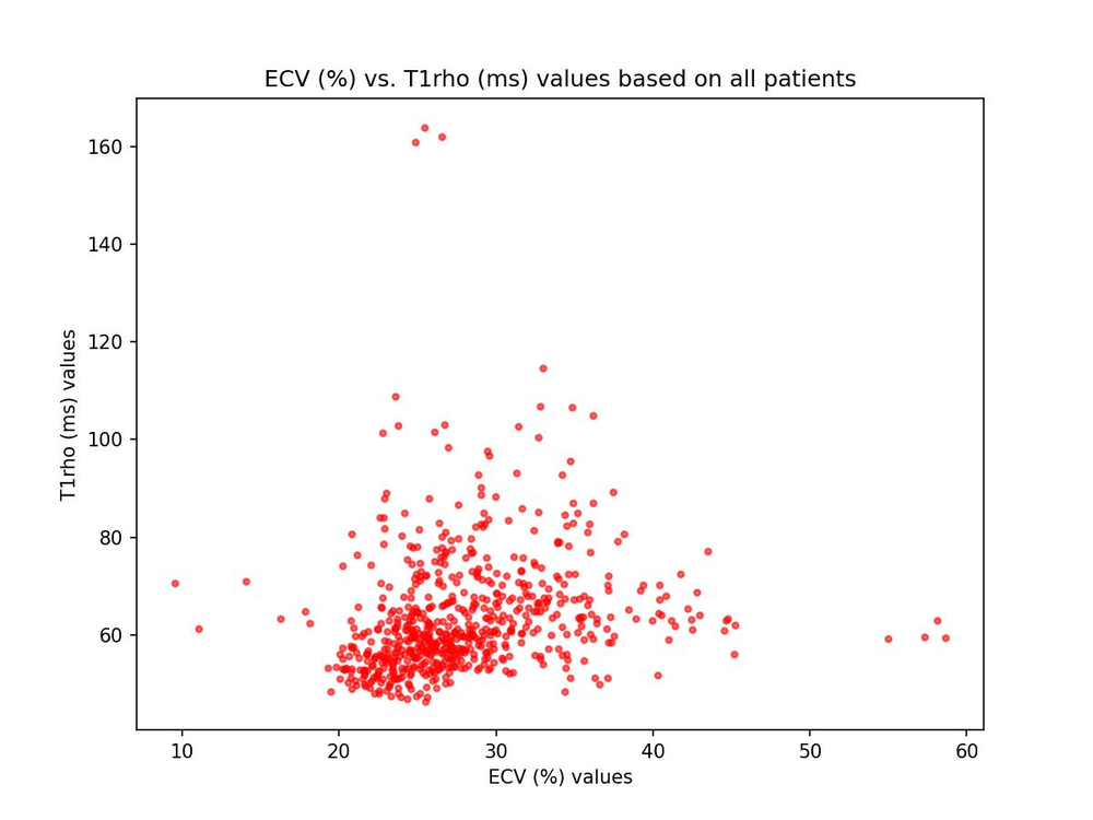
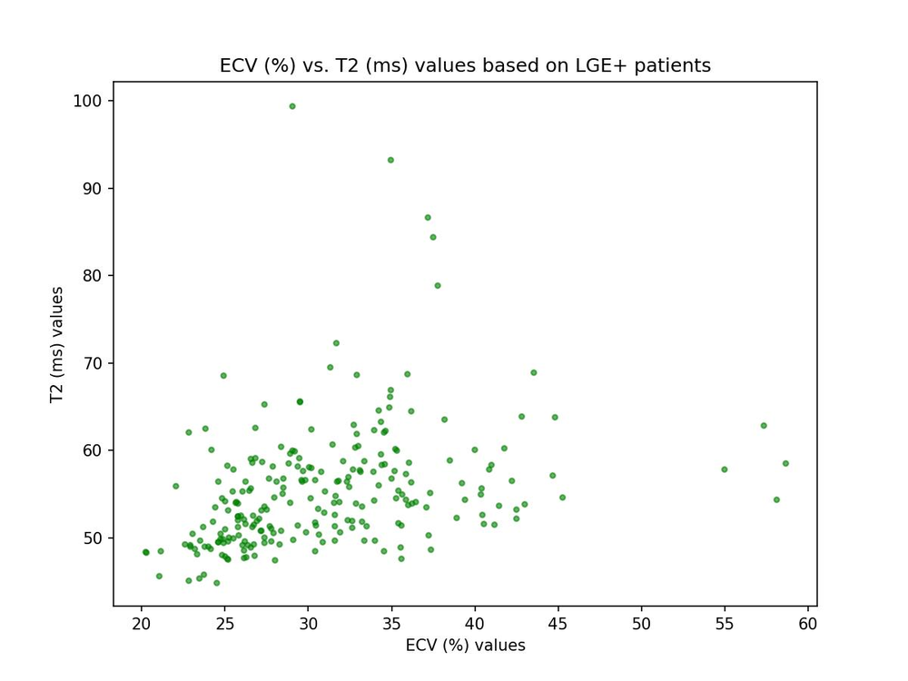
The software calculated a mean value per segment. These means were gathered as tuples of ECV, T1ρ and T2 values in a Python dictionary, mapped to a specific heart segment in each patient. Three scatter plots were then created, comparing two maps at a time. The correlation coefficient r was obtained using pearsonr. Data point pairs were filtered out if one of the elements came from an empty cell, and therefore became a NaN.
A list of 16 patients, out of the 41, had elevations in the LGE map and were classed as LGE-positive (LGE+). This acted as a second filter. The list was used after segmentation, to avoid observation bias.
Data acquisition through regions of interest
Regions of interest (ROIs) were a second way to assess the effectiveness of T1ρ. LGE ROIs were marked where suspected collagen highlights were present, across 70 unselected patients. These 70 patients were not the same as the 16 LGE-positive patients above, although they were also LGE-positive. They had elevations in LGE values, but no clear diagnosis of myocardial fibrosis had been established.
Each LGE ROI was compared to a separate marked region of remote healthy tissue of equal size. The masks were then overlaid onto the T1ρ map of the corresponding slice. Each T1ρ ROI whose mean exceeded the mean of the remote healthy tissue by at least four standard deviations was counted as an elevation detection.
Results
Across the 70 LGE-positive patients, T1ρ detected 85% of the elevations that LGE identified.
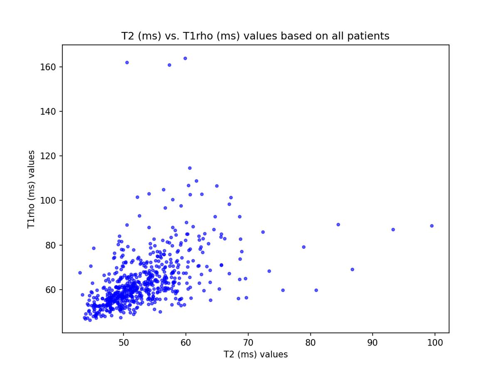
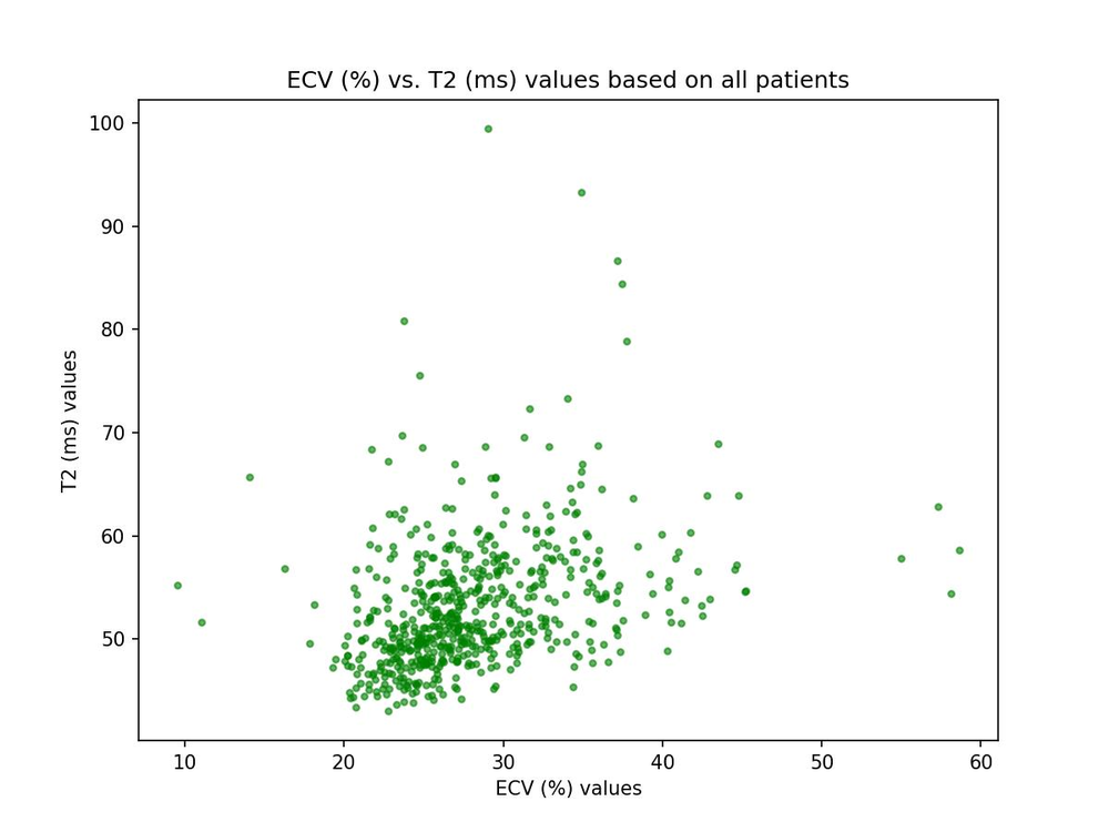
The segment-wise correlations were weaker. The results for all 41 patients are shown below.
| Comparison | r | n |
|---|---|---|
| ECV vs. T1ρ | 0.194 | 656 |
| T2 vs. T1ρ | 0.480 | 608 |
| ECV vs. T2 | 0.340 | 608 |
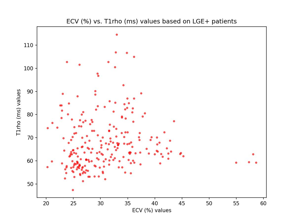
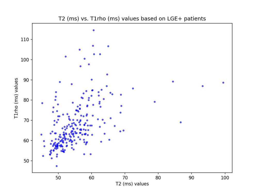
The results for the 16 LGE-positive patients are shown below.
| Comparison | r | n |
|---|---|---|
| ECV vs. T1ρ | 0.047 | 240 |
| T2 vs. T1ρ | 0.478 | 240 |
| ECV vs. T2 | 0.322 | 240 |
All six coefficients fall within −0.5 < r < 0.5.
Discussion
The two analyses point in different directions. The ROI analysis showed that T1ρ identified most of the elevations detected by LGE. The segment-wise correlations showed that ECV, T1ρ and T2 do not measure elevation identically.
LGE is a valid method for diagnosing myocardial fibrosis. The fact that T1ρ detected 85% of the elevations that LGE identified indicates that T1ρ is nearly as accurate as LGE in detecting elevations. However, this sensitivity alone does not establish diagnostic accuracy, since the patients in the data set were unselected.
The strongest correlation in the data set was between T2 and T1ρ: 0.480 across all patients, and 0.478 among LGE-positive patients. This is consistent with what the two maps measure. Both are closely related transverse-relaxation measurements, but the spin-lock RF pulse makes T1ρ more sensitive to water–macromolecule interactions. T1ρ is therefore more similar to T2 than to ECV in what it detects.
Since an elevation does not always equal fibrosis, it is unclear whether using T1ρ over T2 has an advantage in diagnosing myocardial fibrosis.
The correlation between ECV and T1ρ was the weakest of the six, and it weakened further when only LGE-positive patients were analyzed: 0.194 dropped to 0.047. This may be because fewer healthy patients remained in the scatter plot, and healthy values cluster within a narrow interval. The LGE-negative patients created a more centralized area in the plot. Filtering them out led to fewer data points and more widespread values.
Two possible explanations for the weak correlations
The first is that these maps contain different measurements, so they should not be expected to correlate linearly, as the Pearson coefficient r assumes. ECV measures extracellular volume, T2 varies with water content, and T1ρ captures microscopic changes in tissue structure.
The second is that outliers in the scatter plots created a weak correlation. These outliers could have been caused by blood pools surrounding and within the myocardium, which yielded values approaching 150 ms for T1ρ. Since bullseye plots compute the mean for a segment, the blood pools may have been included.
Limitations
The 16-part segmentation was performed semi-automatically. The center of the septum was marked once for multiple slices. If each slice was slightly rotated, for example from movement of the scanned patient, the software may have performed the segmentation incorrectly. This leads to the wrong segment of the heart being displayed as another in the bullseye plot data. A segment containing myocardial fibrosis might then appear healthy, which would invalidate the accuracy of T1ρ in detecting elevations.
Additionally, the position of the mark could not be transferred between image stacks, so the segmentation between stacks may have been shifted. This could not be standardized.
Blood pools might also have been included in the manual isolation of the left ventricle. This potentially contributed to inflated values in T2, T1ρ and ECV, creating outliers. In the data set, the apical slices typically had high values because of blood pools.
Comparison with past studies
Bustin et al. (2021) also used ECG-triggered, bSSFP breath-held MRIs, and also compared T1ρ maps to LGE maps. Their patients were selected: 23 patients with suspected myocardial fibrosis, 15 of them LGE-positive. They used LGE as the reference for T1ρ remote and injured ROIs, and reported 93% sensitivity. The 85% found here, from a larger and unselected group, supports their result.
Van Oorschot et al. calculated r between ECV and T1ρ based on marked ROIs, and obtained 0.66. This is a stronger correlation than the 0.047 to 0.194 found here for the same pair. The difference is methodological: they compared ROIs, whereas this study compared segment means. Mean values from segmentation can therefore yield weaker correlations, since averaging a whole segment dilutes a focal lesion into the surrounding healthy tissue.
Future research
- Shift the epicardial and endocardial borders further, for example by 15% or 20%, while keeping the currently marked myocardium data. If the outliers disappear, the borders were drawn too far outside the true myocardium and included too much blood.
- Ignore the apical slices for each image stack, since they contained the most blood. Scar tissue may be present in those slices, which would reduce the data set.
- Mark ROIs in each map rather than computing mean values per segment. A factor of increase could be calculated by dividing the mean ROI value by the remote healthy tissue mean value. This would establish how clearly the fibrotic tissue is visible between maps. Marking ROIs can, however, introduce observer bias.
- Include the T1 relaxation map in the comparison, for a more definitive picture of how T1ρ compares with established methods.
- Take possible sex-related variations in T1ρ values into account, as C. Han et al. did. Patient sex could be extracted from the MRI metadata.
- Perform a specificity analysis, which would require a list of selected patients with diagnosed myocardial fibrosis alongside unselected patients. Without it, this study measures elevation detection rather than diagnosis.
- Use a larger sample size. The scatter plots did not all have the same number of points.
Conclusion
The maps T2, T1ρ and ECV did not always detect the same elevations, as shown by the weak correlations: all coefficients fell within −0.5 < r < 0.5. T1ρ appears promising, since it detected 85% of the elevations LGE found across 70 LGE-positive patients. It still needs more statistical evidence before it can act as an alternative to contrast agents in clinical settings, because it correlates more weakly with ECV than with T2, both for LGE-positive patients and for all patients.
The weak correlations could stem from systematic errors in the myocardial segmentation, and from outliers caused by blood being included in the segmentation. A stronger version of this study would use more patients, tighter segmentation borders, and ROIs instead of segment means.
Resources
- PDFFull report: Quantitative Cardiac T1ρ MRI: Segmentation and Multi-modal Comparison — 20 pages, with all figures and references
- SoftwareSegment Research by Medviso, used for segmentation and bullseye analysis
- ProgramRays – Research Academy for Young Scientists
AI use and acknowledgements
AI never had access to any of the patient images, or to the spreadsheets based on extracted patient data. Claude Opus 4.8 was used to generate the Python code that read the Excel file and extracted the map values into a dictionary, to debug the scatter-plot code, to rewrite repeated plotting blocks into one reusable function, and to generate the LaTeX code for the five-panel figure. The full disclosure is in the report.
Thanks to my supervisor Pontus Pandurevic for guidance well beyond the standard mentorship weeks; to Albert Meurling Wipf and Kasper Johansson for detailed feedback on the report; to my teachers Katarina Roxström Lindquist and Niklas Schild; to the Rays organisers; and to Beijerstiftelsen, Jacob Wallenbergs Stiftelse and Hierta-Retzius Stipendiefond, who support the program.